Planning with SBPL: Example in X, Y, Theta State Space
This tutorial will go through a simple example of loading in an environment (the Willow Garage floorplan), then generating a plan from a specified start and goal.
As described in the previous tutorial, planning with search-based methods have two parts - representing the problem as a graph, then solving the graph with graph-search methods. SBPL has two objects it uses for these two roles - the environment and the planner. The code below shows the initialization of an environment in the (x, y, theta) state space. We'll then use the ARA* planner to produce our paths.
Initializing the environment
We'll be using an environment file (specific to EnvironmentXYTHETALAT) that already contains values for all the parameters we need, so you can load them right in. But here's the breakdown of what the XYTheta environment requires.
- discretization(cells): this describes how many cells the environment is descretized into.
- Obsthresh: equivalent to cost_lethal (see section 1.5 of the ROS Wiki)
- Cost_inscribed_thresh: (see section 1.5 of the ROS Wiki)
- Cost_possibly_circumscribed_thresh: (see section 1.5 of the ROS Wiki)
- Cellsize(meters): the length of one edge of a square cell. Multipyling each value in the discretization(cell) line should yield the size of your actual map.
- nominalvel(mpersecs): speed of translational movement
- timetoturn45degsinplace(secs): speed of rotational movement
- start(meters,rads): the start x, y, and theta position
- end(meters,rads): the end x, y, and theta position
- environment: a map of the environment.
The Code
You can find the entire file at this GIST. We'll step through the planxythetalat function.
Perimeter of robot
This function defines a vector of points that describe the perimeter of the robot. The (0,0) point of the robot is the reference location that the planner uses. In this example, the robot is a .01m by .01m robot, with its center at (0,0).
Initializing the environment
This initializes our environment with the information from the environment file, perimeter description, and motion primitive file. There are also functions available to initialize an environment without a file, but this requires a lot of parameters to be passed into the initialization function.
Specifying start and goal state
This sets the desired start and goal states to plan between. A very important detail here is that start_id and goal_id get filled in to be used later. BOTH the environment and planner must have their start and goal set. The environment takes in the continuous coordinate for the start and goal, and the planner takes in the state IDs for the start and goal.
Initializing the planner
Here, we specify the initial epsilon. By default, this will decrement the epsilon by .2 after every solved plan. The search mode of the planner denotes if it quits after the first solution (search_mode = true) or if it continues to try and improve its solution quality until it's out of time (search_mode = false). One other parameter here is the bsearch, which sets whether it is a forward or backward search (searching from start to goal or from goal to start).
Planning
The planner takes in an double limiting how long it has to plan. It returns a vector containing the state IDs for the path. It then prints out some stats that shows how long it took to plan, the solution cost, and the final epsilon it reached.
Writing out solution
While the planner returned a vector of state IDs, this is not what you would feed to a controller - it must be converted back into continuous coordinates. The writeSolution function spits out a text file containing both the discrete and continuous paths. You'll notice that the continuous path has many more points than the discrete path. This is because each motion primitive is composed of many waypoints that are expanded for the continuous path.
Running the code
Once you compile the code, you can run it with
$ ./xytheta [location of willow cfg file] [location of motion primitives file]
In the standard SBPL install, use these files
env_examples/nav3d/willow-25mm-inflated-env.cfg
matlab/mprim/pr2.mprim
(By default, the willow cfg comes as a zip, so you have to unzip it first). This will produce two solution files sol.txt and sol.txt.discrete
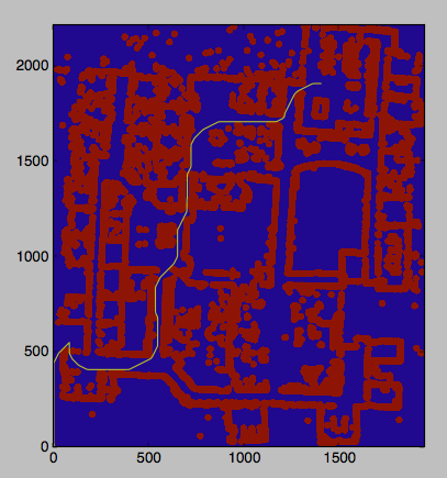
This is the planned path plotted using this python code (depends on matplotlib and numpy). You can run this code with
python visualize.py willow-25mm-inflated-env.cfg sol.txt.discrete